Using PolicyPortfolios
Why PolicyPortfolios?
A policy portfolio is a collection of simple assessments of the presence or absense of state intervention in a specific area (Target) using a concrete state capacity (Instrument). How specific or general the area is, is up to the researcher. How broad or restricted is the collection of assessments is also up to the researcher (Adam, Knill, and Fernandez-i-Marı́n 2017). Using policy portfolios as objects of analysis allows political science to standardize comparitive policy analysis by providing a common ground of policy intervention, and represents a first step of comparing state intervention in different fields of public life.
The package has two sorts of families of functions to deal with policy portfolios.
One set is intended to facilitate the management of portfolio data, either
coming from external sources or once it has been treated in R.
The second set of functions is intended to facilitate the analysis and
visualization of policy portfolio data.
This document requires the following packages:
library(dplyr)
library(tidyr)
library(ggplot2)
Input Data
Structure and characteristics
The input data required for the package to work with is a tidy dataset (Wickham 2014), where every observation is a row and every variable is a column. This makes the data easy to manipulate, model and visualize.
Two fake dataset to show the possibilities of the package has been created, and they can be accessed using the data(PolicyPortfolio) call.
There are two portfolios, one in the energy sector (P.energy) and one in the education sector (P.education).
The energy one looks like follows:
## # A tibble: 12,375 x 7
##    Country  Sector  Year Instrument    Target        p covered
##    <fct>    <fct>  <int> <fct>         <fct>     <dbl>   <dbl>
##  1 Syldavia Energy  2020 Instrument 11 Target 16 0.004       0
##  2 Syldavia Energy  2021 Instrument 11 Target 16 0.003       0
##  3 Syldavia Energy  2022 Instrument 11 Target 16 0.002       0
##  4 Syldavia Energy  2023 Instrument 11 Target 16 0.001       0
##  5 Syldavia Energy  2024 Instrument 11 Target 16 0           0
##  6 Syldavia Energy  2025 Instrument 11 Target 16 0           0
##  7 Syldavia Energy  2026 Instrument 11 Target 16 0           0
##  8 Syldavia Energy  2027 Instrument 11 Target 16 0           0
##  9 Syldavia Energy  2028 Instrument 11 Target 16 0           0
## 10 Syldavia Energy  2029 Instrument 11 Target 16 0           0
## # … with 12,365 more rows
library(PolicyPortfolios)
data(PolicyPortfolio)
P.energyThe object P.energy is a tidy data frame (a tibble) that contains 12,375 rows and 6
variables. 5 of the variables are markers of the case, and only one (“covered”)
is in fact actual data. It indicates whether in the corresponding observation
(defined by “Country”, “Sector”, “Year”, “Instrument” and “Target”) there is
policy intervention (1) or not (0).
In this case, the P.energy dataset contains several countries and traces them
over several years:
levels(P.energy$Country)## [1] "Syldavia" "Borduria" "San Theodoros"unique(P.energy$Year)## [1] 2020 2021 2022 2023 2024 2025 2026 2027 2028 2029 2030The portfolio is in fact the combination of a two-dimensional space composed by policy Targets (“Target”) and the policy Instruments (“Instruments”) than can be used to address such targets.
levels(P.energy$Target)## [1] "Target 16" "Target 17" "Target 18" "Target 19" "Target 20" "Target 21"
## [7] "Target 22" "Target 23" "Target 24" "Target 25" "Target 26" "Target 27"
## [13] "Target 28" "Target 29" "Target 30" "Target 31" "Target 32" "Target 33"
## [19] "Target 34" "Target 35" "Target 36" "Target 37" "Target 38" "Target 39"
## [25] "Target 40"levels(P.energy$Instrument)## [1] "Instrument 11" "Instrument 12" "Instrument 13" "Instrument 14"
## [5] "Instrument 15" "Instrument 16" "Instrument 17" "Instrument 18"
## [9] "Instrument 19" "Instrument 20" "Instrument 21" "Instrument 22"
## [13] "Instrument 23" "Instrument 24" "Instrument 25"The variable “Sector” is only introduced to be able to compare policy sectors. Only policy sectors with the same combinations of Instruments and Targets can be in the same dataset. Otherwise it is understood that the total combination of Targets and Instruments is the one that defines the portfolio. Therefore, is preferable to work with separated portfolios when the space defined by Targets and Instruments is different. For instance, in the portfolio of the education sector, the countries and years are equal as in the energy, but the targets and instruments differ:
levels(P.education$Target)## [1] "Target 1" "Target 10" "Target 11" "Target 12" "Target 13" "Target 14"
## [7] "Target 15" "Target 2" "Target 3" "Target 4" "Target 5" "Target 6"
## [13] "Target 7" "Target 8" "Target 9"levels(P.education$Instrument)## [1] "Instrument 1" "Instrument 10" "Instrument 2" "Instrument 3"
## [5] "Instrument 4" "Instrument 5" "Instrument 6" "Instrument 7"
## [9] "Instrument 8" "Instrument 9"Prepare a dataset with a portfolio structure
The function pp_clean() may help in transforming the data from a
spreadsheet-like format into a tidy format.
By default, it uses a structure coming from the
consensus research
project. Guidelines for external experts to collect data on
social and environmental policies are available, as well as the coding
manual.
An example of a speardsheet collecting data for policy portfolios in the
Consensus project is the following:
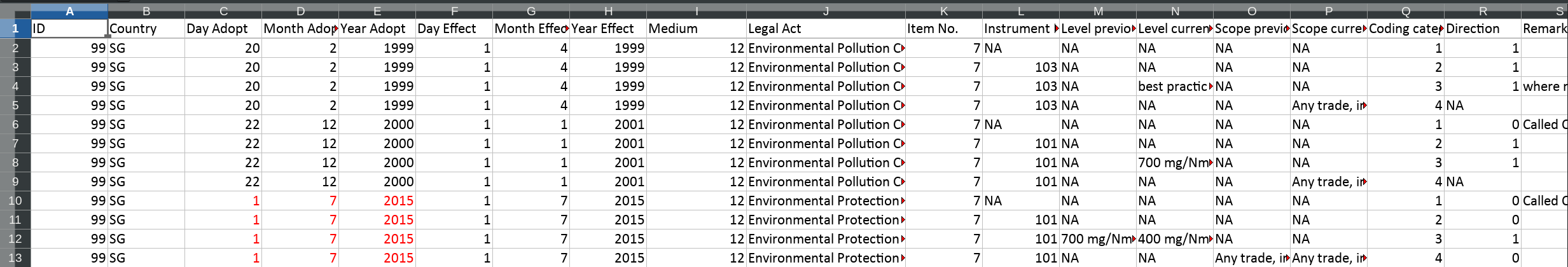
spreadsheet <- read.table(...)
d <- pp_clean(spreadsheet,
              Sector = "Environmental",
              Year.name = "Year.Adopt",
              coding.category.name = "Coding.category",
              Instrument.name = "Instrument.No.",
              Target.name = "Item.No.")

pp_complete()
pp_clean() easily transforms a wide format coming from a spreadsheet into a
tidy object suitable for policy portfolio analysis, doing several checks on the
consistency of the original data and helping to spot inconsistencies and to debug
problems with the coding process.
The coding process involves looking for instances where there is policy
intervention in different scenarios, and therefore in cases (Instruments and
Targets) when even not a single case of policy intervention has been observed
the data would not include such a space. For instance, we may be interested in
recording whether there is policy intervention in, say, providing funds for
schools when there is a disabled student in a clasroom. But if we do not observe
any single case in the portfolio, the final dataset will not contain this
possibility, and therefore we must complete the observed portfolio with the
potential full range of Targets and instruments. THis is achieved with the pp_complete() function.
dc <- pp_complete(d,
                  Instrument.set = full.factor.of.potential.instruments,
                  Target.set = full.factor.of.potential.targets)
One the dataset is cleaned and complete we may proceed to its analysis.
Analyze policy portfolios
One the structure of the tidy dataset required is clear, we can start using the functions to extract information of interest from it.
Summarize portfolios
The main function that summarizes the characteristics of the portfolio is
pp_measures(). It takes a tidy portfolio data frame as input and produces a tidy data frame with entries for all the Countries and Years of the original input plus several measures with their corresponding values.
pp_measures(P.energy)| Country | Sector | Year | Measure | value | Measure.label |
|---|---|---|---|---|---|
| Syldavia | Energy | 2020 | Space | 375.0000 | Portfolio space |
| Syldavia | Energy | 2020 | Size | 0.0187 | Portfolio size |
| Syldavia | Energy | 2020 | n.Instruments | 6.0000 | Number of instruments covered |
| Syldavia | Energy | 2020 | p.Instruments | 0.4000 | Proportion of instruments covered |
| Syldavia | Energy | 2020 | n.Targets | 7.0000 | Number of targets covered |
| Syldavia | Energy | 2020 | p.Targets | 0.2800 | Proportion of targets covered |
| Syldavia | Energy | 2020 | Unique | 6.0000 | Number of unique instrument configurations |
| Syldavia | Energy | 2020 | C.eq | 0.5429 | Equality of Instrument configurations |
| Syldavia | Energy | 2020 | Div.aid | 0.9524 | Diversity (Average Instrument Diversity) |
| Syldavia | Energy | 2020 | Div.gs | 0.8163 | Diversity (Gini-Simpson) |
| Syldavia | Energy | 2020 | Div.sh | 2.5216 | Diversity (Shannon) |
| Syldavia | Energy | 2020 | Eq.sh | 0.6454 | Equitability (Shannon) |
| Syldavia | Energy | 2020 | In.Prep | 1.0000 | Instrument preponderance |
| Syldavia | Energy | 2021 | Space | 375.0000 | Portfolio space |
| Syldavia | Energy | 2021 | Size | 0.0187 | Portfolio size |
The argument id allows to explicitly ask for concrete portfolios, defined by
the elements of the list that is passed.
pp_measures(P.energy, id = list(Country = "Borduria", Year = 2010:2021))## # A tibble: 26 x 6
## Country Sector Year Measure value Measure.label
## <fct> <fct> <int> <fct> <dbl> <fct>
## 1 Borduria Energy 2020 Space 375 Portfolio space
## 2 Borduria Energy 2020 Size 0.016 Portfolio size
## 3 Borduria Energy 2020 n.Instrumen… 5 Number of instruments covered
## 4 Borduria Energy 2020 p.Instrumen… 0.333 Proportion of instruments covered
## 5 Borduria Energy 2020 n.Targets 5 Number of targets covered
## 6 Borduria Energy 2020 p.Targets 0.2 Proportion of targets covered
## 7 Borduria Energy 2020 Unique 5 Number of unique instrument confi…
## 8 Borduria Energy 2020 C.eq 0.5 Equality of Instrument configurat…
## 9 Borduria Energy 2020 Div.aid 0.925 Diversity (Average Instrument Div…
## 10 Borduria Energy 2020 Div.gs 0.778 Diversity (Gini-Simpson)
## # … with 16 more rowsAs a tidy dataset itself, the output of pp_measures() can be easily combined
with other functions to produce figures or tables of interest:
pp_measures(P.energy) %>%
  # Use only a single measure of interest
  filter(Measure == "Size") %>%
  # Use only observations with a concrete time period
  filter(Year > 2022) %>%
  # Convert the long format into wide, and therefore "Size" becomes a column
  spread(Measure, value) %>%
  # Pass this object to "ggplot()" and produce a time series of portfolio "Size"
  ggplot(aes(x = Year, y = Size, color = Country)) +
    geom_line()
Figure 1: Temporal evolution of the size of portfolios, by country.
In this sense, the output produced by the functions in the package is directly suitable for being used by ggplot2, based on the grammar of graphics (Wilkinson et al. 2005), which empowers R users by allowing them to flexibly crate graphics (Wickham 2009).
pp_measures(P.energy) %>%
  # Pick the two measures of portfolio diversity
  filter(Measure %in% c("Div.gs", "Div.sh")) %>%
  # Use only the last year observation
  filter(Year == max(Year)) %>%
  # Select only the relevant variables required to produce the output table
  select(Country, Measure.label, value) %>%
  # Transform the long object into wide, so that every Measure is one column
  spread(Measure.label, value) %>%
  # Sort by decreasing Shannon diversity
  arrange(desc(`Diversity (Shannon)`))
## # A tibble: 3 x 3
## Country `Diversity (Gini-Simpson)` `Diversity (Shannon)`
## <fct> <dbl> <dbl>
## 1 Borduria 0.910 3.57
## 2 Syldavia 0.816 2.52
## 3 San Theodoros 0.75 2The current list of Measures that pp_measures() produces is the following:
| Measure | Measure.label |
|---|---|
| Space | Portfolio space |
| Size | Portfolio size |
| n.Instruments | Number of instruments covered |
| p.Instruments | Proportion of instruments covered |
| n.Targets | Number of targets covered |
| p.Targets | Proportion of targets covered |
| Unique | Number of unique instrument configurations |
| C.eq | Equality of Instrument configurations |
| Div.aid | Diversity (Average Instrument Diversity) |
| Div.gs | Diversity (Gini-Simpson) |
| Div.sh | Diversity (Shannon) |
| Eq.sh | Equitability (Shannon) |
| In.Prep | Instrument preponderance |
Visual display of portfolios
The function pp_plot() produces a visual representation of the two-dimensional
space of policy Targets (horizontal axis) and Instruments (vertical axis) and
whether such space is covered by policy intervention or not.
It requires a single policy portfolio, and therefore if the original tidy
dataset includes several years or countries, this must be explicitly stated
using the argument id:
pp_plot(P.energy, id = list(Country = "Borduria", Year = 2025))
Figure 2: Visual representation of the Energy portfolio of Borduria in 2025, using the pp_plot() function and defining a specific country and year in a list in the id argument.
By default pp_plot() produces a caption with the source of the data, a
subtitle with the measures of the portfolio and the boxes are side by side, but
all these features can be tunned in the arguments. Check the documentation for
more details.
Several options can be passed to tune the visual aspect of the portfolio,
namely spacing, that includes separation between the boxes, dropping the
subtitle with subtitle and changing the default caption with caption.
pp_plot(P.education,
        id = list(Country = "Borduria", Year = 2030),
        spacing = TRUE,
        subtitle = FALSE, caption = NULL)
Figure 3: Visual representation of the Energy portfolio of Borduria in 2025, using the pp_plot() function and defining a specific country and year in a list in the id argument.
Finally, pp_report() is an encompassing function that generates a report in
html with detailed descritive analysis of the portfolios, both considering them
individually as well as comparatively (comparing countries or measures).
pp_report(P.energy)It also contains several arguments that can help in the analysis, but the defaults are expected to be comprehensive and meaningful.
Other possibilities
It is possible to transform the tidy policy portfolio data frame into an array,
in case that operations in a matrix-like style are required to be performed.
This can be achieved with the pp_array() function:
A <- pp_array(P.energy)

# Get the dimensions:
# 3 is Country
# 1 is Sector
# 11 is Year
# 15 is Instrument
# 25 is Target
dim(A)
## [1] 3 1 11 15 25Final remarks
PolicyPortfolios facilitates the generation of measures of policy portfolios
and its visualization, as well as the cleaning process of such datasets. It only
requires, as a central component, a tidy dataset that defines whether certain
policy space defined by a Target and an Instrument is covered by policy
intervention or not.
Development
The development of PolicyPortfolios (track changes, propose improvements, report bugs) can be followed at https://github.com/xfim/PolicyPortfolios.
References
Adam, Christian, Christoph Knill, and Xavier Fernandez-i-Marı́n. 2017. “Rule Growth and Government Effectiveness: Why It Takes the Capacity to Learn and Coordinate to Constrain Rule Growth.” Policy Sciences 50 (2): 241–68.
Wickham, Hadley. 2009. Ggplot2: Elegant Graphics for Data Analysis. Use R! Springer-Verlag. https://books.google.es/books?id=bes-AAAAQBAJ.
———. 2014. “Tidy Data.” Journal of Statistical Software 59 (1): 1–23. https://doi.org/10.18637/jss.v059.i10.
Wilkinson, L., D. Wills, D. Rope, A. Norton, and R. Dubbs. 2005. The Grammar of Graphics. Statistics and Computing. Springer-Verlag.