The emergence of Regulatory Regionalism: transnational networks and the diffusion of regulatory agencies within regions

Abstract
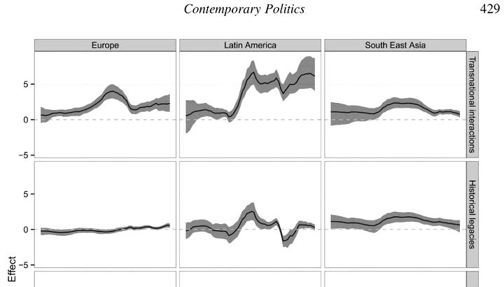
The regulatory regionalism approach has increasingly claimed that a new mode of regional governance is emerging globally. Regional policy regimes, developed in broad social and economic territorial areas, affect the internal transformation of the state. The authors plan to provide comprehensive empirical evidence about the emergence of worldwide regulatory regionalism by identifying how regulatory agencies have diffused very successfully within the regional level in recent decades. The paper aims to identify, using an original methodological design, the ways in which such diffusion of agencies occurred, as this may have theoretical relevance for the study of regulatory regionalism. The authors’ hypothesis suggests that transnational political interactions in each regional cluster triggered agency diffusion, contributing to the development of the regulatory state within the countries of each region. To test this hypothesis, the authors employed a data set of regulatory agencies including the OECD (Organisation for Economic Co-operation and Development), and most Asian and Latin American countries (+59) from 1950 to 2007, for 15 sectors related to finance, risks, utility and competition. Bayesian data analysis was used to estimate the parameters of interest.
"The emergence of Regulatory Regionalism: transnational networks and the diffusion of regulatory agencies within regions" is an article by Xavier Fernández-i-Marín and Jacint Jordana published at Contemporary Politics in 2015. This webpage contains supplemental online material that complements the published paper with DOI: 10.1080/13569775.2015.1010776.
Technical documentation
The supplemental online material (pdf, 60K) contains technical documentation, including agencification coverages by country, description of the database, results not shown in the main paper (time evolution and country differences) and models for robustness checks.
Dataset
The dataset contains three columns: Country, Sector and Creat-11. The first two are case indicators, whereas Creat-11 refers to the year of creation of a regulatory agency checked in 2011. The date of creation, its meaning and its implications, are described in the online material of another paper of the authors, published in 2011 at Comparative Political Studies with David Levi-Faur (“The Global Diffusion of Regulatory Agencies: Channels of Transfer and Stages of Diffusion”). The first observations look as follows:
"Country","Sector","Creat-11"
"Argentina","Competition",1980
"Argentina","Electricity",1992
"Argentina","Environment",
"Argentina","Financial Services",1935
"Argentina","Food Safety",1992
"Argentina","Gas",1992
"Argentina","Health",1996
"Argentina","Insurance",1937
"Argentina","Pensions",1993
Code
The code for the first model (no regional / time differences) in the BUGS/JAGS declarative language follows:
model {
  for (i in 1:d.I) {
	d.y.perc.betareg[i] ~ dbeta(a[i], b[i])
        a[i] <- mu[i] * phi[d.ic[i]]
        b[i] <- (1 - mu[i]) * phi[d.ic[i]]
        logit(mu[i]) <-
	         (theta[d.time[i]] )
	       + (beta[1] * log.gdp.cap.sc[i])
	       + (beta[2] * igo.number.sc[i])
	       + (beta[3] * d.W.dist.sc[i])
               + (beta[4] * d.W.imp.sc[i])
               + (beta[5] * d.W.igo.sector.economic.sc[i])
               + (beta[6] * d.W.hist.sc[i])
  }
phi factor
for (c in 1:d.C) {
phi[c] ~ dgamma(0.001, 0.001)
}
theta by time
theta[1] ~ dnorm(0, 0.001)
for (yr in 2:d.Y) {
theta[yr] ~ dnorm(theta[yr-1], tau.theta)
}
tau.theta <- pow(sigma.theta, -2)
sigma.theta ~ dunif(0, 10)
control variables
beta[1:6] ~ dmnorm(b0[1:6], B0[1:6,1:6])
missing values
for (i in 1:d.I) {
log.gdp.cap.sc[i] ~ dnorm(0, 1)
}
}
The code for the second model (regional differences, but not time differences) in the BUGS/JAGS declarative language follows:
model {
  for (i in 1:d.I) {
	d.y.perc.betareg[i] ~ dbeta(a[i], b[i])
        a[i] <- mu[i] * phi[d.ic[i]]
        b[i] <- (1 - mu[i]) * phi[d.ic[i]]
        logit(mu[i]) <-
	         (theta[d.time[i]] )
	       + (beta[1, d.id.r[i]] * log.gdp.cap.reg.sc[i])
	       + (beta[2, d.id.r[i]] * igo.uniregional.number.sc[i])
	       + (beta[3, d.id.r[i]] * d.W.dist.reg.sc[i])
               + (beta[4, d.id.r[i]] * d.W.imp.reg.sc[i])
               + (beta[5, d.id.r[i]] * d.W.igo.uniregional.sector.economic.sc[i])
               + (beta[6, d.id.r[i]] * d.W.hist.sc[i])
  }
phi factor
for (c in 1:d.C) {
phi[c] ~ dgamma(0.001, 0.001)
}
theta by time
theta[1] ~ dnorm(0, 0.001)
for (yr in 2:d.Y) {
theta[yr] ~ dnorm(theta[yr-1], tau.theta)
}
tau.theta <- pow(sigma.theta, -2)
sigma.theta ~ dunif(0, 10)
control variables by region
for (r in 1:d.R) {
#beta[1:5, r] ~ dmnorm(b0[1:5], B0[1:5,1:5])
for (b in 1:6) {
beta[b, r] ~ dnorm(b0[b], tau.beta[b])
}
}
for (b in 1:6) {
b0[b] ~ dnorm(0, 0.01)
tau.beta[b] <- pow(sigma.beta[b], -2)
sigma.beta[b] ~ dunif(0, 10)
}
missing values
for (i in 1:d.I) {
log.gdp.cap.reg.sc[i] ~ dnorm(0, 1)
}
}
The code for the third model (regional and time differences) in the BUGS/JAGS declarative language follows:
model {
  for (i in 1:d.I) {
	d.y.perc.betareg[i] ~ dbeta(a[i], b[i])
        a[i] <- mu[i] * phi[d.ic[i]]
        b[i] <- (1 - mu[i]) * phi[d.ic[i]]
        logit(mu[i]) <-
	         (delta[d.time[i]] )
	       + (beta[1, d.id.r[i]] * log.gdp.cap.reg.sc[i])
	       + (beta[2, d.id.r[i]] * igo.uniregional.number.sc[i])
	       + (theta[1, d.id.r[i], d.time[i]] * d.W.dist.reg.sc[i])
               + (theta[2, d.id.r[i], d.time[i]] * d.W.imp.reg.sc[i])
               + (theta[3, d.id.r[i], d.time[i]] * d.W.igo.uniregional.sector.economic.sc[i])
               + (theta[4, d.id.r[i], d.time[i]] * d.W.hist.sc[i])
  }
phi factor
for (c in 1:d.C) {
phi[c] ~ dgamma(0.001, 0.001)
}
delta by time
delta[1] ~ dnorm(0, 0.001)
for (yr in 2:d.Y) {
delta[yr] ~ dnorm(delta[yr-1], tau.delta)
}
tau.delta <- pow(sigma.delta, -2)
sigma.delta ~ dunif(0, 10)
theta by time
for (r in 1:d.R) {
theta[1:4, r, 1] ~ dmnorm(t10[1:4], T10[1:4, 1:4])
for (yr in 2:d.Y) {
theta[1:4, r, yr] ~ dmnorm(theta[1:4, r, yr-1], R[r, 1:4, 1:4])
}
R[r, 1:4, 1:4] ~ dwish(Omega[1:4, 1:4], 4)
}
control variables by region
for (r in 1:d.R) {
beta[1:2, r] ~ dmnorm(b0[1:2], B0[1:2,1:2])
}
for (b in 1:2) {
b0[b] ~ dnorm(0, 0.001)
}
missing values
for (i in 1:d.I) {
log.gdp.cap.reg.sc[i] ~ dnorm(0, 1)
}
}